Predicting kernel spectra powerlaw exponents from raw data statistics
This is a technical note on kernel theory. Venture in at your own risk!
My collaborators and I recently put out a paper called Predicting kernel regression learning curves from raw data statistics in which, among other things, we show how to map from the data PCA stats to the eigenfunctions and eigenvalues of a broad swath of rotation-invariant kernels. It’s a surprising result, both mathematically and empirically: the formulas we find are very simple, and they predict very well for both synthetic Gaussian datasets and image datasets like CIFAR-10. This has given me real hope that we can deal with the problem of data in the fundamental science of deep learning.
At about the same time, Arie Wortsman and Bruno Loureiro published a paper that takes up a very similar topic! They also ask about the mapping from data covariance stats to kernel eigenvalues, and where we discuss the same questions, we find agreeing answers. They’re particularly interested in powerlaws (while we’re more spectrum-agnostic), and they’d like to know: if the data covariance eigenvalues decay as a powerlaw with exponent $\alpha$, with what exponent do the kernel eigenvalues decay?
This is a great question, well-motivated by recent developments in practical machine learning and attempts to explain them. The data decay exponent is a more fundamental object, but the kernel eigenvalue decay exponent is the more practically important one. It’s a good question to ask how they’re linked. In this blogpost, I’ll review their answer, propose an alternative perspective with some experiments to back it up, and discuss what I see as important open questions.
Review: the answer of Wortsman and Loureiro (2025)
Let the data be sampled $\mathbf{x} \sim \mathcal{N}(\mathbf{0}, \boldsymbol{\Gamma})$ with $\boldsymbol{\Gamma} = \mathrm{diag}(\gamma_1, \ldots, \gamma_d)$. Let the data covariance eigenvalues be $\gamma_i = i^{-a}$ with exponent $a > 1$. (We could add a constant of proportionality — that is, $\gamma_i = \gamma_0 i^{-\alpha}$ — but this only changes the results trivially, so I’ll assume $\gamma_0 = 1$ to keep things simple.) The data dimension $d$ will be very large; for the purposes of this blogpost, we will let it be infinite.
Wortsman and Loureiro find that the kernel eigenvalues asymptotically decay as $\lambda_j \sim j^{-a}$ — that is, the kernel spectral decay exponent is the same as the data covariance decay exponent. They give nice formal bounds that imply this, and they also give a beautiful characterization of the spectrum when $d$ is finite and $a < 1$, which is very mathematically satisfying (if less practically relevant, since in with real data one almost always finds that $a> 1$).1
Turning to experiment: can we see this?
I find that, when studying machine learning, it’s always a good idea to go check your results against experiment. So what happens if we try this prediction with a real kernel function? To try this, I drew $n = 10^4$ samples of Gaussian data with eigenvalues $\gamma_i \propto i^{-a}$ with exponent $a= 1.5$ and unit trace $\sum_i \gamma_i = 1$, with data dimension $d = 10^4$. I then computed the spectrum of a Gaussian kernel $K_\sigma(\mathbf{x}, \mathbf{x}’) = e^{-\frac{1}{2 \sigma^2} |\mathbf{x} - \mathbf{x}’|^2}$ with different kernel widths $\sigma$ over this dataset and plotted the spectrum. Here’s what I found:
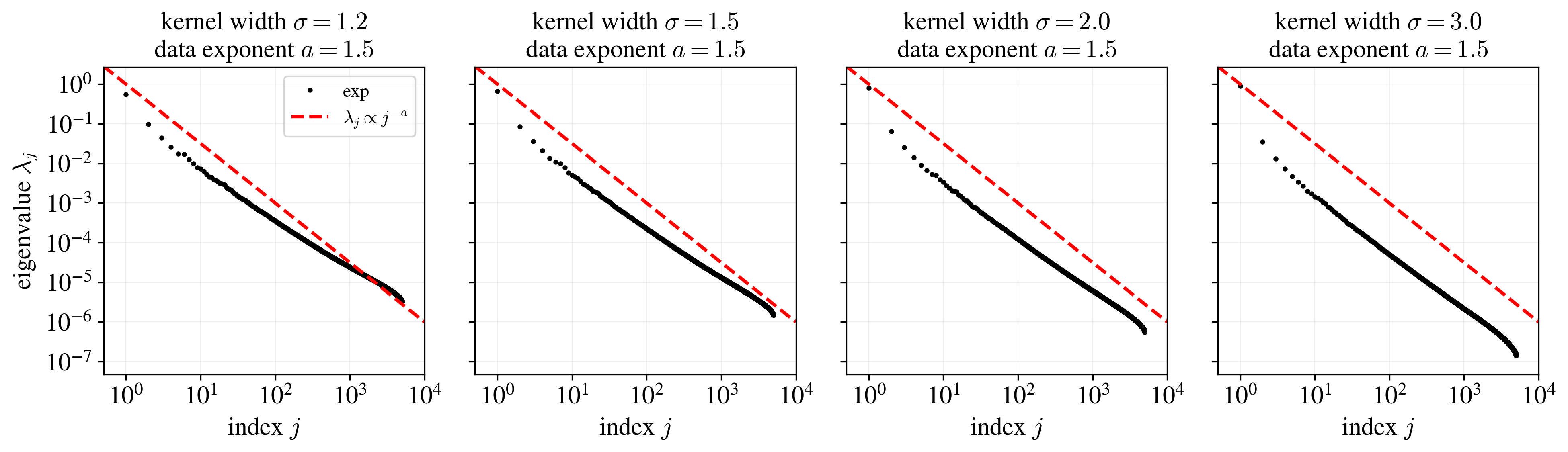
A few observations. First, the spectrum is… kind of a nice powerlaw in the middle? But the transient effects at the head and finite-size effects at the tail make it annoying to tell; we’ll have to deal with these. Second, even if you squint, it’s hard to argue that the decays all look like powerlaws with $a = 1.5$. Third, the decay rates actually seem to change: the plots with larger $\sigma$ seem to have a faster decay and a larger exponent. This wasn’t in the prediction of Wortsman and Loureiro (2025). What gives, and can we predict the decay rates we actually see here?
The HEA: an alternative approach
I’m going to argue that, yeah, their answer that “the spectral decay rate is always $a$” is probably right asymptotically as you look very deep into the spectrum, but you’ll often have to look prohobitively far into the spectrum before you approach that decay rate. To do so, I’ll introduce a mathematical tool for getting the precise shape of the decay curve, even at small values of the index $j$.
The main technology we’ll use to do this is the Hermite eigenstructure ansatz (HEA) from our paper. I won’t go through it in detail here; see the paper or Joey’s blogpost. The main point we’ll use here is that the HEA gives nice, explicit formulae for the kernel eigenvalues in terms of some kernel-derived coefficients (which are basically Taylor series coefficients). For the Gaussian kernel with width $\sigma$, we have $c_\ell = e^{-\frac{1}{\sigma^2}} \cdot \sigma^{-2 \ell}$. Then
\[\left\{ \lambda_j \quad \text{for all } \quad j \in \mathbb{N} \right\} = \left\{ c_{|\boldsymbol{\alpha}|} \cdot \prod_i \gamma_i^{\alpha_i} \quad \text{for all } \quad \boldsymbol{\alpha} \in \mathbb{N}_0^d \right\}. \tag{HEA}\]In words: the set of all kernel eigenvalues (the left-hand side) equals the set enumerated on the right, where the enumeration runs over all multi-index vectors $\boldsymbol{\alpha} \in \mathbb{N}_0^d$ and each choice of $\boldsymbol{\alpha}$ gives a certain monomial of the data covariance eigenvalues $\gamma_i$. This is the deep idea from our paper, and it unifies a lot of other cases with known kernel spectra. I won’t explain why it’s true here, but there is a pretty satisfying derivation we give in our paper.2
The HEA isn’t exact, and it isn’t perfect, but in our paper, we show that it’s empirically very accurate in basically every case we hoped it would be, including Gaussian-data cases like the one we’re studying here. Let’s check: I’ll add the theoretical spectrum predicted by simple enumeration of the HEA eigenvalues to the plots.
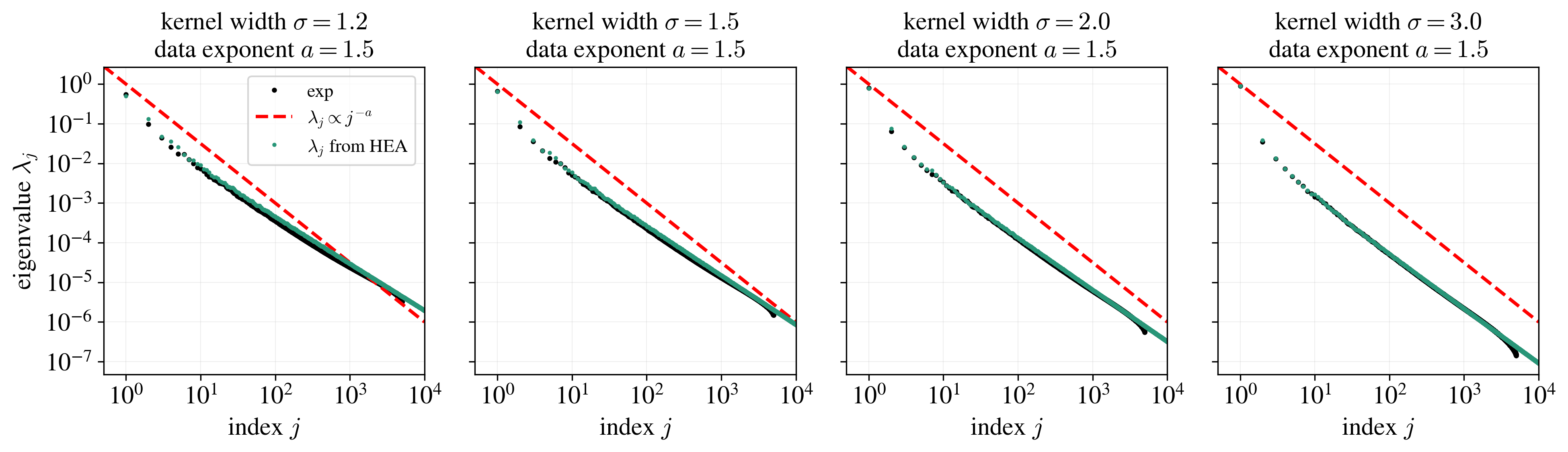
Pretty good! It’s not perfect, but it’s pretty close, and the discrepancy in the tails is probably due to finite-size effects in the experiment. I trust the HEA more there, and the HEA seems to show a fairly nice powerlaw that spans several decades! It looks reasonably like the eigenvalues actually follow a powerlaw with a different slope $a’ \neq a$. I didn’t draw those lines because I wasn’t totally sold, but I’m close to buying it.
To proceed, let’s just assume the HEA gives us the exact spectrum and ask what that implies.
From the HEA to spectral decay?
Now that we just have a closed-form construction for the kernel spectrum, all that remains is to look at its decay w.r.t. index. The right-hand side of the HEA is a sum over multi-indices —- it naturally takes the shape of a $d$-dimensional array —- so the challenge is just flattening this set down to a one-dimensional sorted list.
Treated as a discrete math problem, this is difficult. I’m a physicist, though, so when I see a problem like this, I’ll first try a continuum approximation to the sum and see if that works.
We want a function for $\lambda(j)$, the eigenvalue at index $j$. It turns out it’s easier to go after $j(\lambda) = \#[\textrm{eigenvalues } \ge \lambda]$ and then invert it. To get $j(\lambda)$, a decent idea is to do a Laplace’s method “saddle point” analysis: most of the total number of eigenvalues less than $\lambda$ will occur at or near a particular eigenvalue order $\ell_*$, and Taylor-expanding the multiplicity locally around $\ell_*$ turns out to be a useful idea.
It turns out that ChatGPT can just do this whole calculation if you throw it the problem setup. After some minutes of thinking, it reports that:
\[\lambda(j)\ \propto \ f(j; \sigma, a) \equiv j^{-a}\;\exp\!\Big(2a\,\sqrt{r\,\log j}\Big)\;(\log j)^{-\,\frac{3a}{4}},\]where $r = \Big(\sigma^{-2}\gamma_1\Big)^{1/a}$. So does this work? Let’s add it to the plot:
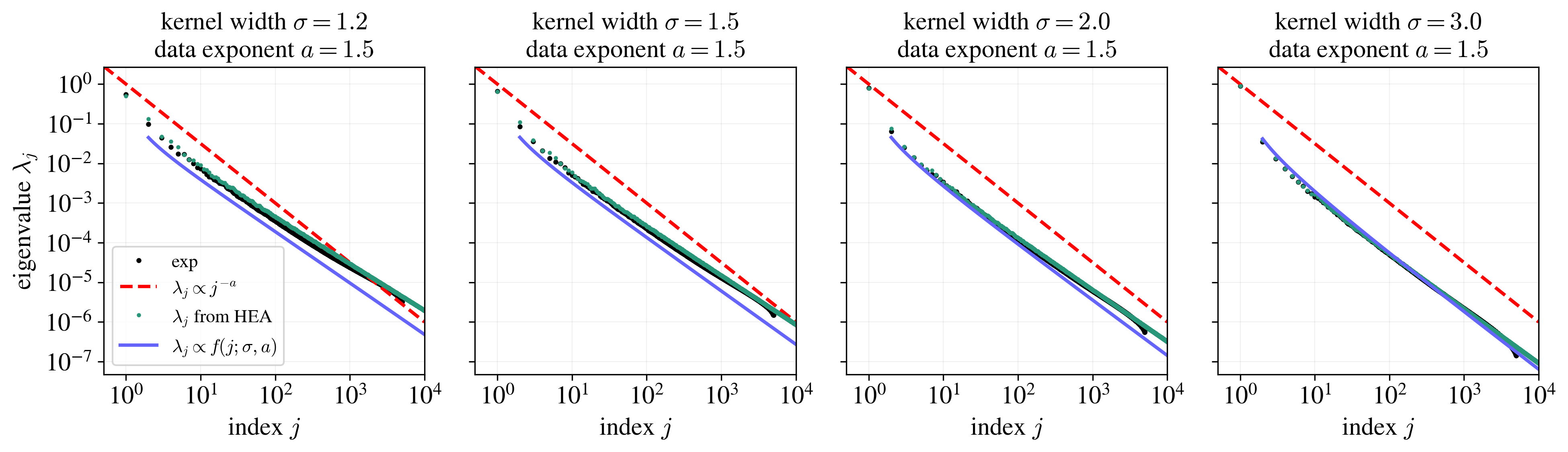
Not really. I’m not sure why. Even after adding more terms (i.e. considering a higher-order expansion around the saddle point), it doesn’t work. It’s possible that GPT’s calculation was just wrong; I haven’t checked in detail (and that’s a first thing to do were I to take up this problem seriously). It’s better than just assuming a powerlaw with exponent $a$, though.
Let’s ignore the discrepancy and study the function $f(j; \sigma, a)$ anyways. A first observation is that it actually does asymptotically decay like $j^{-a}$. A second observation, though, is that it can take a really, really long time to get there. Here’s a plot of the slope on a log-log plot:
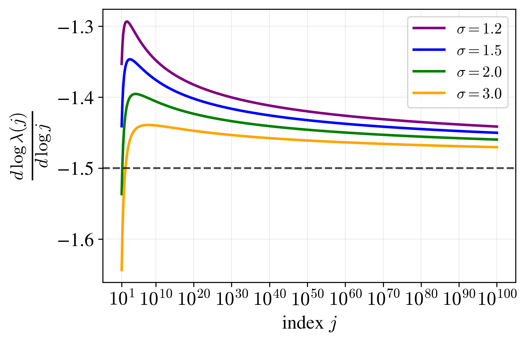
Slope on a log-log plot of $\lambda(j) = f(j; \sigma, a)$ with $a = 1.5$. Note that it takes an extremely long time to converge to the asymptotic slope of $-a = -1.5$!
When $\sigma$ isn’t particularly big, sometimes it takes up to $j \sim 10^{100}$ to actually get close to a decay rate of exponent $a$. Perils of asymptotic analysis! Really makes me suspect that all the power laws we see in machine learning are actually just locally powerlaws, and over enough orders of magnitude, they’ll change.
What now?
I’d say the big open question here is: given that the HEA eigenvalues look pretty good, what analysis can you do on top of them? It’s probably not the right idea to jump all the way to the asymptotic decay rate. Instead, it’ll probably turn out that the decay rate is roughly constant for the first several decades (say, from $10^1$ to $10^6$), and that’s the more interesting value to predict, since it’s the one we’ll see in experiments.
-
The second half of Arie and Bruno’s paper is a treatment of how the data spectrum drives generalization in KRR, which is one step beyond the kernel spectrum! I’m just not discussing it because I’m focused on the powerlaw spectrum question here. ↩
-
For an alternative approach, you can actually see Arie and Bruno’s Proposition 1 — they find essentially the HEA’s eigenvalue prescription in almost the same language! Their result involves constant-factor bounds on the eigenvalues (while we give the eigenvalues including constant factors), but this price is paid in exchange for their actually proving their result rigorously, where we do not except in two limiting cases. Which of these you’ll want to use probably depends on your style! If you just want a formula to try in experiments, our presentation is probably preferable. If you want to prove theorems or build rigorous mathematical foundations, our results should be a good guide for the intuition, but their analysis is probably a better place to build from. ↩