The polynomial features of random neural networks
The language of polynomials is beautiful and well-developed: millenia of work have furnished a rich, deep theory that spans analysis and algebra, with basics we teach to children and high reaches still under development. The language of neural network features has not yet been written, but it promises to be beautiful: empirics show that hidden features can represent complex concepts and form striking circuitry. Fortunately, more and more results in fundamental deep learning theory suggest that the language of polynomials might actually be the language of hidden features, at least to a substantial fraction. How wonderful if we could fathom the depths of learning and cognition with polynomial algebra!
My (biased) favorite example of this confluence of languages comes from my recent paper, which will appear at ICLR in April. We performed a first-principles study of the inductive biases of simple learning methods and found that (a) they treat real image datasets as Gaussian blobs, and that (b) learning on these blobs decomposes into independent learning of Hermite polynomial coefficients. What falls out is a surprisingly simple and beautiful theory of inductive bias which makes excellent (i.e. correct) predictions of test-time performance on different tasks. Just look at these curves which we predict using our polynomial language:
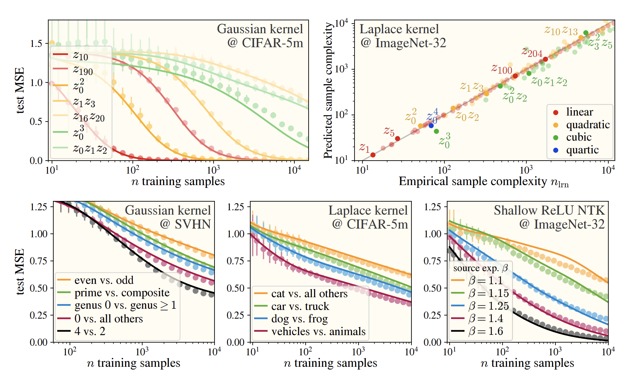
A figure from our paper Karkada*, Turnbull* et al. (2026) showing extremely good prediction of kernel regression learning curves from minimal dataset statistics.
You might be thinking: reading papers is hard, and that one looks quite technical. You might then be wondering: is there a simpler way to see how polynomial language arises in this context? If that’s so, dear reader, then you have clicked on the right blogpost. The purpose of this note is to walk through the deep underlying reason why Hermite polynomials arise in the description of neural network hidden features.
Setup
Consider a data vector $\mathbf{x} \in \mathbb{R}^d$ and a nonlinear transformation $\mathbf{h}(\mathbf{x}) := \sigma(\mathbf{W}\mathbf{x})$ which embeds it in a feature space. Here $\mathbf{W} \in \mathbb{R}^{n \times d}$ is a linear transformation and $\sigma(\cdot)$ is an elementwise nonlinearity. For the picture we want to develop, it’s enough to let $\mathbf{W}$ be random with $W_{ij} \sim \mathcal{N}(0, \frac{\alpha}{d})$. No polynomials yet: since we didn’t require $\sigma$ to be a polynomial, each hidden activation $h_i(\mathbf{x})$ is a complicated, nonpolynomial function.
Dot-product kernels have polynomial features
The key idea is that, given one assumption, these secretly are polynomial features up to rotation. After a suitable orthogonal transformation on $\mathbf{h}(\mathbf{x})$, we get polynomial features. This is most easily seen with kernel language: take a second data vector $\mathbf{x}’$ and consider the feature kernel $K(\mathbf{x}, \mathbf{x}’) := \frac{1}{n} \langle \mathbf{h}(\mathbf{x}), \mathbf{h}(\mathbf{x}’) \rangle$. Let us make the following assumption on this kernel:
From Assumption A, it follows immediately that the hidden features are equivalent up to rotation to polynomial features:
where we have defined the prismatic operation $\boldsymbol{\psi}_\mathbf{c}(\mathbf{x})$ containing all monomial features of $\mathbf{x}$ (more on that to come in a future paper). When the data is Gaussian and the level coefficients $c_\ell$ decay quickly, Gram-Schmidt orthogonalization of the elements of this prismatic feature vector gives the Hermite polynomials (!!) as kernel eigenfunctions. It turns out real image data is often Gaussian enough for the Hermite polynomials to be a good approximation to the kernel eigensystem. This is pretty much the whole story of our paper.
When can we take Assumption A?
The problem with Assumption A is that, strictly speaking, it’s false. Random feature kernels do not take this exact dot-product form, even in the infinite-width limit. Fortunately, we can often make that assumption, and it’s not too wrong.
Let’s return to the random feature kernel above. As we take width $n \rightarrow \infty$ and take the average over hidden neurons and their associated Gaussian weights, we get the kernel
This is precisely the neural network Gaussian process (NNGP) kernel of Lee et al. (2017). Remember that we’re initializing our random weights as $W_{ij} \sim \mathcal{N}(0, \frac{\alpha}{d})$, so that’s where the $\frac{\alpha}{d}$ comes in.
The NNGP kernel $K_{\sigma,\alpha}(\mathbf{x},\mathbf{x}’)$ is rotation-invariant: that is, it admits the form
\[K_{\sigma,\alpha}(\mathbf{x},\mathbf{x}') = K_{\sigma,\alpha}(\|\mathbf{x}\|^2, \|\mathbf{x}'\|^2, \langle\mathbf{x},\mathbf{x}'\rangle).\]However, it is not a true dot product kernel; those first two norm arguments are real.1 That said, we can ignore the first two arguments if we know they do not vary over our dataset. For example, if we know that every data vector we will care about lies on a sphere: $\lVert\mathbf{x}_i\rVert = r \ \forall i$, then we can neglect the first two arguments, and we are left with a dot-product kernel.
Of course, it’s a rare case when our data’s exactly on a sphere, but it’s often the case that the data roughly concentrates in norm, as is the expectation in high dimension. In such cases, we approximately get a dot-product kernel, and the eigensystem is approximately built from Hermite polynomials. This approximation is often very reliable in practice: in our paper, we show that assuming concentration of norm allows us to predict the eigensystem of CIFAR-10 with great accuracy (see learning curves above).
To show how robust this assumption is, it’s worth noting that the data norms of CIFAR-10 really don’t concentrate very tightly; see the figure below. This poor concentration is still good enough to do theory that assumes the norm concentrates. At least in many cases, this a robust assumption.
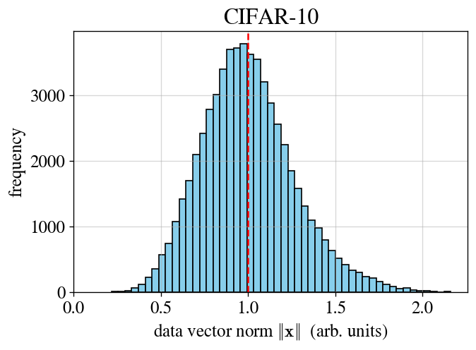
The data vector norms for CIFAR-10 don't concentrate tightly around their mean (dashed line). Nonetheless, eigensystem calculations based on an assumption of concentration of norm work remarkably well.
If I’m honest, I don’t really know why we didn’t have to take corrections involving the width of this distribution into account. It’s probably something that some future theory paper will have to go back and understand. Moving forward, though, we can reliably take Assumption A for real image datasets, which gives us a dot-product kernel, polynomial features, and a Hermite eigensystem.
The remainder of this post consists of some technical notes on how to calculate kernel level coefficients. They probably won’t interest you unless (and until) you need them.2
Activation function $\rightarrow$ kernel coefficients on the sphere
Let’s assume our data lies on a sphere: $\lVert\mathbf{x}_i\rVert = r$. Our NNGP kernel is then
\[K_{\sigma,\alpha}(\mathbf{x},\mathbf{x}') = K_{\sigma,\alpha,r}(\langle \mathbf{x}, \mathbf{x}' \rangle) = \sum_{\ell \ge 0} \frac{c_\ell}{\ell!} \langle \mathbf{x}, \mathbf{x}' \rangle^\ell.\]How do the level coefficients $c_\ell$ depend on $(\sigma, \alpha, r)$? There is a simple answer: computing the Gaussian expectation above, we find that
\[c_\ell = \frac{\ell!}{r^{2\ell}} \left( \mathbb{E}_{z \sim \mathcal{N}(0,1)} \! \left[ h_\ell(z) \ \sigma\!\left( r\sqrt{\tfrac{\alpha}{d}}\, \cdot z \right) \right] \right)^2,\]where $h_\ell(z) = \frac{1}{\sqrt{\ell!}} \text{He}_\ell(z)$ is the $\ell$-th normalized probabilist’s Hermite polynomial. In words, we’re extracting the $\ell$-th Hermite coefficient of the function $z \mapsto \sigma\left( r\sqrt{\tfrac{\alpha}{d}}\, \cdot z \right)$. That prefactor of $r\sqrt{\tfrac{\alpha}{d}}$ makes a lot of sense: it’s the standard deviation of the (Gaussian!) preactivations fed into the activation function $\sigma(\cdot)$. Hermite decompositions of a rescaled activation function often show up in this corner of theoryland.3
This is a powerful result: if you know the Hermite decomposition of $\sigma(\cdot)$, then you know the level coefficients of your kernel and the relative weights of the different orders of monomial features. The Hermite decompositions of common activation functions (e.g. $\text{ReLU}$) can be worked out in closed form. Moreover, a lot can be learned from symmetries and taking note of which Hermite coefficients are exactly zero. For example, $\sigma = \tanh$ is odd, so it will lack all even coefficients: $c_{2\ell} = 0$. In a weirder case, $\sigma = \text{ReLU}$ equals a linear function plus an even function, so it has $c_\ell = 0$ for $\ell = 3, 5, 7, \cdots.$ This particular pathology of $\text{ReLU}$ has cropped up many times in my research.
Activation function $\rightarrow$ kernel coefficients near the origin
Now things are going to get somewhat subtle. So far, when we’ve talked about concentration of norm, we’ve really meant that the norm of the data vectors concentrates in a relative sense, not in an absolute sense. That is, we care that
\[\frac{\max_i \|\mathbf{x}_i\|}{\min_j \|\mathbf{x}_j\|} \approx 1, \qquad \text{not that} \qquad \max_i \|\mathbf{x}_i\| - \min_j \|\mathbf{x}_j\| \approx 0.\]However, there is a very important solvable limit in which the data vectors concentrate in norm absolutely but not relatively. This is the limit in which the data vectors all have small norm: $\lVert\mathbf{x}_i\rVert \ll 1$. If all the vectors have the same small norm (e.g., $\lVert\mathbf{x}_i\rVert = \lVert\mathbf{x}_j\rVert = r \ll 1$), or the variation is also small in a relative sense, then we recover the case above. However, what we really want is an analysis valid for all $\mathbf{x} \in r B^{d}$, where $r \ll 1$ and $B^d$ is the $d$-ball.
The method of attack here is direct: simply examine the kernel $K_{\sigma,\alpha}(\lVert\mathbf{x}\rVert^2, \lVert\mathbf{x}’\rVert^2, \langle\mathbf{x},\mathbf{x}’\rangle)$ and naively (Taylor-)expand it for small $\lVert\mathbf{x}\rVert^2, \lVert\mathbf{x}’\rVert^2$. Upon trying this, one quickly makes a few observations:
- It is not always possible to take this expansion analytically. For example, the Laplace kernel $e^{-\lVert\mathbf{x} - \mathbf{x}’\rVert}$ is not smooth around zero in these arguments.
- This smoothness is related to the smoothness of the activation function $\sigma$ around zero: if the activation function is analytic around zero, so is the kernel.
- The derivatives of $\sigma$ determine the coefficients of the kernel’s Taylor series.
In particular, one finds that so long as the activation function is analytic (on all of $\mathbb{R}$) and integrates nicely against Gaussians, the NNGP kernel is given exactly by
In the above, $\sigma^{(k)}(0)$ denotes the $k$-th derivative of $\sigma$ evaluated at zero. When the norms are small ($\lVert\mathbf{x}_i\rVert, \lVert\mathbf{x}_j\rVert \ll 1$) the $q, q’ = 0$ terms dominate those with $q, q’ \ge 1$, and we can heuristically approximate
\[K_{\sigma,\alpha}(\mathbf{x},\mathbf{x}') \approx \sum_{\ell \ge 0} \frac{c_\ell}{\ell!} \langle \mathbf{x}, \mathbf{x}' \rangle^\ell \qquad \text{where} \qquad c_\ell = \left(\frac{\alpha}{d} \right)^\ell \cdot \left( \sigma^{(\ell)}(0) \right)^2.\]This is a main result in what I think of as “wide kernel theory”: the study of kernels which are much wider than the data distributions on which they’re evaluated, often leading to great simplifications and nice polynomial forms.4
Some examples for different choices of $\sigma$
Here we report values of these small-norm level coefficients for different activation functions. Note that care must be taken to correctly incorporate the right power of $\alpha/d$.
Derivatives of different activation functions.
I used GPT to help with some of the math here. I’ve sense-checked all of it, and the final results have already fed into successful experiments I’ve run, so I feel pretty confident in this, but I own any errors.
-
It can be proven that only in the trivial affine case $\sigma(z) = a z + b$ is the NNGP kernel exactly a dot-product kernel. ↩
-
Looking at you, Joey Turnbull. ↩
-
This connection between the Hermite decomposition of the activation function and the level coefficients of the resulting NNGP kernel was first pointed out by Daniely et al. (2016), and the NTK version was later given by me and friends in Simon et al. (2021). I no longer believe in the importance of that paper’s central story, but our Theorem 3.1 is still great. ↩
-
Worth noting that, while I think this heuristic approximation will be pretty much fine, there are some subtleties involved; in particular, since kernels are inverted when they’re used, dropping a small term can change that inverse unless it falls “in the shadow” of larger terms. Dropping these terms might change learning on a small number of norm-sensitive target functions. ↩