eight ways to get Gabors from the same whitened natural images, each with a time slider over 100 checkpoints
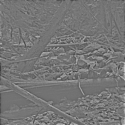
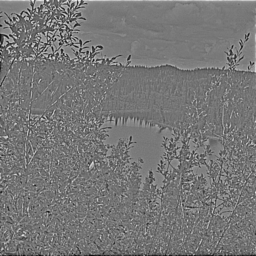
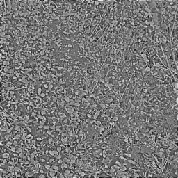
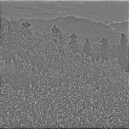
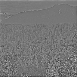
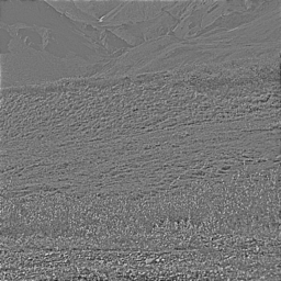
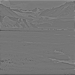
Olshausen's ten whitened natural images; what every method here is trained on
Master dataset. Olshausen's ten whitened 512 × 512 natural images (IMAGES.mat from the sparsenet code at the Redwood Center), already whitened and low-pass filtered with \(R(f) = f\,e^{-(f/f_0)^4}\), \(f_0 = 200\) cycles/image. Every method sees \(16 \times 16\) patches drawn uniformly from these images and nothing else; no further preprocessing except where the method's description says so. Each tab shows one method: a description with its knobs counted, then the basis functions at 100 checkpoints log-spaced in the method's own time, laid out in the order they settled (top-left settled first; a unit has settled when it stays within \(|\cos| \ge 0.9\) of its final form). Gabor-ness is measured by a least-squares fit of a 2-D Gabor to each final basis function, reported as \(R^2\) (1 = exactly a Gabor).
The images. 10 images of 512 × 512 pixels (shown at 190 px). Pixel values have mean -0.000, standard deviation 0.28, range -2.0 to 2.9; the per-image standard deviations run from 0.12 to 0.45. There are 2,381,440 possible 16 × 16 patch positions (4-pixel border excluded), but only about 10,240 non-overlapping ones: this is a small dataset, and every method here sees the same patches many times over.
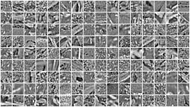
Patches. 144 random 16 × 16 patches, each scaled to its own range. A single pixel has excess kurtosis 3.3; a random unit direction in the 256-dimensional patch space has median excess kurtosis 2.9. Everything below is about finding the directions that are far more kurtotic than that.
The images are low-pass filtered, so the last ~30 of 256 directions carry under \(10^{-4}\) of the top variance and a few eigenvalues are numerically negative. ICA-type methods whiten, which divides by these: hence the floor, and hence \(M = 192\) as the honest 'complete' dimension for them (99.85% of the variance). The Olshausen-Field model does not whiten and is unaffected.
What could run live in the browser
Each time below is for one complete run as shown on its tab: the whole training, all units, from random start to the final basis
(not one unit, not one step). Assumptions: WebGPU, the browser's compute API, running on the laptop's own GPU (an Apple M-series chip; no server,
no node) at a realistic 1 TFLOP/s sustained; the whole dataset resident on the GPU; the inner loops written as a handful of kernels.
Symbols: \(N\) = number of training patches (20,000-100,000 here; a 16 × 16 patch is 256 pixels), \(d\) = dimensions kept after PCA
(64-192; the dimension the ICA-type methods work in), \(K\) = number of units learned (basis functions, ICA components or neurons; 256 here),
\(B\) = minibatch size, \(T\) = number of steps or iterations. The arithmetic column counts floating-point operations for the run, from those
sizes; one dense multiply of an \(N imes d\) matrix by a \(d imes K\) matrix is \(2NdK\) flops.
Plain JavaScript without WebGPU is 100-1,000x slower; only projection pursuit and FastICA are comfortable there.
Findings (2026-10-28 evening; every battery of the day is in)
What was found. Every method that pushes past second-order statistics gives Gabors on this dataset; the clean ones need no
sparsity machinery at all.
ICA, all units at once (01c): FastICA with the \(\log\cosh\) or \(u e^{-u^2/2}\) contrast gives median Gabor \(R^2\) 0.93-0.95 at every
dimension tried (64 to 256), converged in ~300 iterations; half the units are within 0.9 cosine of their final form by iteration ~100.
The kurtosis contrast (\(u^3\)) gives the same at \(M = 64\) (0.89) and collapses at \(M \ge 192\) (0.24-0.31): the floored near-null
PCA directions are heavy-tailed, and a fourth moment finds them first. Kurtosis is the fragile statistic; \(\log\cosh\) is not.
Projection pursuit, one unit at a time (01d): \(R^2\) 0.85-0.87 for \(\log\cosh\)/exp at every \(M\): slightly worse than the symmetric
version, because each later unit is squeezed into the orthogonal complement of the earlier ones. Units take 20-100 iterations each.
Nonlinear Hebbian rule (01e), one learning rate: works. With minibatches of 100 the result is Gabors plus SGD noise
(\(R^2\) 0.77 at \(M = 192\), still drifting at 20,000 steps); at \(M = 64\) minibatches of 10,000 give 0.90 with 90% of units above 0.8,
settled by ~1,000 steps. But at \(M = 192\) the big batch makes it worse (0.33): without the SGD noise the cubic rule converges to
the rare high-frequency outlier directions, the same thing kurtosis ICA does at that dimension. The same rule with a saturating \(\tanh\) output learns nothing
(\(R^2\) 0.21-0.23 at every batch size and step size, which is what random directions score): on whitened data \(\tanh\) is linear
where it matters, and a linear Hebb rule has no preference between directions. The superlinear part is what selects Gabors.
AGF utility maximisation (01g), the two-layer-network step: on whitened 64- and 128-dimensional patches, 256 neurons climbing
\(\mathbb E|w\cdot z|^\alpha\) for \(\alpha\) = 2.25, 2.5, 3 all land on localised Gabors (\(R^2\) 0.95-0.97, 95-100% above 0.8) but on only
7-8 (M = 64) or 13-14 (M = 128) distinct ones, nearly all vertical: the utility landscape has very few maxima, and independent
neurons pile onto them. \(\alpha < 2\) with \(|z|^\alpha\) gives junk (\(R^2\) 0.13), as it must: those maximisers are the sub-Gaussian
directions. \(\mathrm{relu}(z)^\alpha\) and \(\mathrm{sign}(z)|z|^\alpha\) are a little less Gabor-like (0.8-0.9) but find 2-6x more
distinct directions, and the odd statistic works below \(\alpha = 2\) (\(\mathrm{sign}(z)|z|^{1.25}\): 0.80, 78 distinct). At
\(M = 192\), \(\alpha = 3\) gives long oriented bars spanning the patch (23 distinct, \(R^2\) 0.68), and \(\alpha \ge 4\) finds the
amplified near-null directions (\(R^2\) 0.25), the same failure as kurtosis ICA. \(\mathrm{relu}(z)^4\) at \(M = 64\): 51 distinct, \(R^2\) 0.86.
The \(\alpha\) and \(M\) scan is in 01g.
Infomax (01f): \(R^2\) 0.92 for learning rates 0.01-0.03 at 30,000 minibatch steps; 0.001 is simply unconverged (0.4-0.7).
Olshausen-Field (01b): the simplest version wins. Unit-norm columns, Cauchy prior, no gain homeostasis: \(R^2\) 0.94 with 80% of
256 units above 0.8 at 20,000 batches, half the units settled by ~11,000. Every run with sparsenet.m's variance homeostasis is worse at
the same step count (\(R^2\) 0.25-0.56 at \(M = 256\); 0.76 at 192, 0.89 at 128, 0.87 at 64): ~90 Gabors learned, the rest still noise with gains driven to
~0.1, i.e. the homeostasis slows the unused units down rather than recruiting them. The \(e^{-u^2}\) prior gives 0.87. The 100,000-step
homeostatic run is pending. Getting sparsenet.m's version to run at all needed the code read closely: the variance average updates once
per sample, the prior weight is \(\beta\) not \(\beta/\sigma\), inference starts from the least-squares projection.
What this says about the driving question. The directions a superlinear nonlinearity "sees" on whitened images are exactly the
Gabors, provided the nonlinearity grows slower than \(|z|^4\): \(|z|^{2.5}\) is already enough, and the result is as Gabor-like as ICA's.
What a plain utility climb does not give is a basis: it gives the few best directions, repeatedly. Something must push neurons
apart (orthogonalisation in ICA, the residual in AGF proper, the reconstruction term in sparse coding). The sequential-residual AGF runs
(agfseq_*) test whether a constant target's residual is enough to do that; with \(y = 1\) the fitted amplitudes are tiny
(the \(|z|^3\) feature has a huge variance relative to a constant), so the residual barely moves and the answer is probably no.
Why vertical: settled. The same climb on the images rotated by 90 degrees, or transposed, puts 199-219 of the 256 neurons on
horizontal edges and none on vertical ones (orientation of the top clusters 87-93 degrees instead of 177-180), with the same
\(R^2\) 0.97 and 9-11 distinct directions. The preference follows the pictures: vertical edges are the most kurtotic directions in these
ten images (tree trunks, stems), and a pure utility climb reports the single most kurtotic direction, many times over. That is the
clearest statement so far of what a superlinear nonlinearity sees and what it misses.
The sequential (residual) AGF with a constant target does not fix the collapse. With \(y = 1\) the least-squares amplitudes of
the activated \(|z|^\alpha\) features are ~\(10^{-3}\), the residual stays at 0.99-1.00, and the later neurons climb the same landscape:
1-4 activations in 20,000 steps, 5-60 distinct directions at \(M = 192\). A target with structure (the image itself, i.e. reconstruction)
is what makes the residual informative; that is the next experiment (cost: minutes).
A changing residual gives diversity, not (yet) a Gabor basis (01h). With the patch itself as the target, the 256 neurons end on
256 distinct directions in every run: the residual does push them apart. But the directions are only partly Gabors: the first 32 to
activate score \(R^2\) 0.77-0.80, and it falls to 0.36-0.38 for the last 32, which climb a residual with little structure left in it
(\(\mathrm{relu}(z)^2\) at \(M = 64\) removes 79% of the variance; \(\mathrm{sign}(z)|z|^{2.5}\) 74%; \(|z|^3\)-type features only 10-40%).
The fitted output vectors are no better (0.5-0.6). So on this evidence the Gabor shape comes from the statistic (the first maxima of a
superlinear utility on the raw data), and the residual supplies the spread; a joint gradient flow on the active set, or a smaller step
schedule, may give both at once. Unverified.
The PCA control behaves (01g, "unwhitened"). On data projected onto the top \(M\) principal components with their variances kept,
256 neurons climbing \(|z|^2\), \(|z|^{2.5}\) or \(|z|^3\) all converge to a single direction, the first principal component (its utility
equals the top eigenvalue to three digits), and \(\mathrm{relu}(z)^2\) to three. So without whitening a superlinear utility sees the
variance, not the shape; the whitening is what lets the shape of the distribution decide. On the patch target with \(\alpha = 1\) (linear),
the activated neurons span the principal subspace in an arbitrary rotation (199 distinct, residual 0, \(R^2\) 0.62), as linear
reconstruction must.
The homeostatic model does not catch up (01b). At 100,000 steps (5x longer) sparsenet.m's version at \(M = 256\) is at
\(R^2\) 0.30 with 39% of units above 0.8, against 0.25 and 34% at 20,000: ~100 Gabors and the rest pinned at gains ~0.06, for good. The
\(M\) scan at 20,000 steps is 0.87, 0.89, 0.76, 0.25-0.56, 0.21 for \(M\) = 64, 128, 192, 256, 512, and slower or less noisy learning
helps it (\(\eta\) = 0.1: 0.69; batch 1,000: 0.81). The no-homeostasis version at 0.94 stands.
Iterated AGF, one neuron at a time (01i): Gabors first, then the residual runs out of them. James's version: a neuron climbs the
reconstruction residual's utility to convergence (8 random starts, keep the best), is frozen, the output vectors are refitted, repeat.
The first 32 neurons are clean Gabors, \(R^2\) 0.85-0.89 for \(\mathrm{sign}(z)|z|^\alpha\) with \(\alpha\) = 1.5-2.5 and 0.76-0.86
for \(\mathrm{relu}(z)^{2\text{-}2.5}\) at \(M = 64\), the same quality as the best-of-256 neurons on 01h and as ICA. After that the quality
falls steadily to ~0.3 for the last 32: once the kurtotic structure is explained, what is left of a whitened patch is close to Gaussian
and has no preferred directions, and the climb returns whatever local maximum it finds. The eight starts agree with each other
(min/max utility 0.97-1.0) for \(\alpha \le 2\), i.e. the utility has essentially one maximum, and disagree (0.3-0.5) for \(\alpha \ge 3\),
i.e. many local maxima. How much of the variance the sequence eats depends on \(\alpha\): with 256 neurons, \(\alpha = 1\) (linear) leaves 0
at \(M = 64\) (PCA, as it must; the unwhitened \(\alpha = 1\) run eats it in eigenvalue order), \(\alpha\) = 1.5-2 leaves 4-21%,
\(\alpha = 2.5\) 25-55%, \(\alpha \ge 3\) 60-94% (a cubic feature has a huge variance relative to what it explains, so least squares
gives it a tiny weight). So this version does look like projection pursuit, and it gives the same Gabors as projection pursuit for its
first few dozen units; the difference is that reconstruction, unlike orthogonalisation, stops supplying Gabors once the sparse structure
is gone. A first version of this run had a step budget of one radian per neuron and never reached a maximum (\(R^2\) 0.45-0.6 even for
the first neurons); that was a schedule bug, not physics, and is noted in the run log.
Unexplained / to do. The number of
distinct maxima of the constant-target utility grows with \(M\) (8 at 64, 13 at 128, 14 at 160) and with the one-sidedness of the
nonlinearity (\(\mathrm{relu}(z)^3\): 20 at \(M = 64\), 28 at 128); what sets it is not understood.
Olshausen-Field with unit-norm basis functions (no gain homeostasis), M = 256 on 16 x 16 patches
Method. Olshausen & Field (1996): a generative model \(x = A a + \text{noise}\) with a sparse prior on the
coefficients. Per patch, infer \(a\) by minimising \(E(a) = \tfrac{1}{2\sigma_n^2}\|x - Aa\|^2 + \tfrac{\beta}{\sigma}\sum_i \log(1 + a_i^2/\sigma^2)\)
(Cauchy prior; here 200 accelerated-gradient steps from \(a = 0\)); then take a Hebbian step on the basis,
\(A \leftarrow A + \eta\,(x - Aa)\,a^{\top}/B\), and rescale each column so that its coefficient's running variance drifts towards a
target (sparsenet.m's gain homeostasis). Knobs: \(\sigma_n^2 = 0.01\), \(\beta = 2.2\), \(\sigma = 0.316\), \(\eta = 1\), batch
\(B = 100\), variance goal 0.1 with rates 0.001 and 0.02, plus the inference budget: eight, all at sparsenet.m's values.
Time = learning steps (batches of 100 patches). Shown first is the simpler variant that drops the homeostasis and just keeps every
column at unit norm (five knobs): at 20,000 steps it is the best Olshausen-Field run of the battery; the homeostatic runs are in the table.
Shown: run sn_M256_nohomeo: M = 256, 20,000 steps, beta = 2.2, eta = 1.0, homeo = False, prior = cauchy, infer_steps = 200; median Gabor \(R^2\) of the final basis 0.94; 750 s on one GPU.
learning steps (batches)
Basis functions (each tile scaled to its own max |value|, grey = 0), in settle order: top-left settled first. Drag the slider (log-spaced in time) or press play.
Gabor fits of the first and last units to settleAll pilot variants of this method
One row per pilot run (jobs/pilot.txt). R² is the Gabor-fit quality of the final basis functions.
symmetric FastICA on PCA-whitened patches, log cosh contrast
Method. Hyvärinen's FastICA. Centre the patches and PCA-whiten them to \(M\) dimensions, \(z = V(x - \mu)\);
look for an orthogonal \(W\) whose rows give maximally non-Gaussian projections \(s = Wz\), by the fixed-point iteration
\(w \leftarrow \mathbb{E}[z\,g(w^{\top}z)] - \mathbb{E}[g'(w^{\top}z)]\,w\) on every row at once, followed by symmetric
decorrelation \(W \leftarrow (WW^{\top})^{-1/2}W\). \(g = \tanh\) (the \(\log\cosh\) contrast), \(g(u) = u^3\) (kurtosis) or
\(g(u) = u e^{-u^2/2}\). Shown: the basis functions, i.e. the columns of \(V^{-1}W^{\top}\) back in pixel space. Knobs:
the number of PCA components \(M\) and the contrast function: two. No learning rate. Time = fixed-point iterations, each a
pass over a fixed set of 100,000 patches. The images' low-pass filter leaves the last ~30 of 256 principal directions with
\(< 10^{-4}\) of the top variance, so whitening to all 256 amplifies noise (a run at \(M = 256\) without a floor went NaN);
the eigenvalues are floored at \(10^{-4}\) of the largest.
Shown: run ica_M192_logcosh: M = 192, 500 steps; median Gabor \(R^2\) of the final basis 0.95; 66 s on one GPU.
fixed-point iterations
Basis functions (each tile scaled to its own max |value|, grey = 0), in settle order: top-left settled first. Drag the slider (log-spaced in time) or press play.
Gabor fits of the first and last units to settleAll pilot variants of this method
One row per pilot run (jobs/pilot.txt). R² is the Gabor-fit quality of the final basis functions.
FastICA by deflation: find the most non-Gaussian direction, fix it, find the next orthogonal to it
Method. The same fixed-point update as 01c, but on a single direction \(w\) until it stops moving
(\(1 - |w_{\text{new}}\cdot w| < 10^{-6}\)), orthogonalised against the directions already found; then the next one. This is
projection pursuit (Friedman & Tukey) with FastICA's contrast as the projection index, and it is the literal version of
"find one, let it solidify, find the next". The layout here is the order of discovery. Knobs: \(M\), the contrast,
and a convergence tolerance: three. Time = cumulative one-unit iterations; the per-unit charts below say how many
iterations each unit took.
Shown: run pp_M192_logcosh: M = 192, 200,000 steps; median Gabor \(R^2\) of the final basis 0.87; 114 s on one GPU.
one-unit iterations (cumulative)
Basis functions (each tile scaled to its own max |value|, grey = 0), in settle order: top-left settled first. Drag the slider (log-spaced in time) or press play.
Gabor fits of the first and last units to settleAll pilot variants of this method
One row per pilot run (jobs/pilot.txt). R² is the Gabor-fit quality of the final basis functions.
Is the fixed-point iteration gradient descent on a loss? (James, 2026-10-29.) Nearly: it is an approximate Newton step for
the stationary points of \(J(w) = \mathbb E[G(w\cdot z)]\) on the unit sphere, with \(G\) the contrast and \(z\) the whitened patch. With a
multiplier for the constraint, \(\mathcal L = \mathbb E[G(w\cdot z)] - \tfrac{\beta}{2}(|w|^2 - 1)\), the gradient is \(\mathbb E[z\,g(w\cdot z)] - \beta w\) and
the Hessian \(\mathbb E[zz^{\top} g'(w\cdot z)] - \beta I\), which FastICA approximates by \((\mathbb E[g'(w\cdot z)] - \beta)\,I\) because the data are white.
The Newton step is then proportional to \(\mathbb E[z\,g(w\cdot z)] - \mathbb E[g'(w\cdot z)]\,w\), the update above, and its fixed points are the
stationary points of \(J\) on the sphere (maxima and minima alike). Plain gradient ascent on the same \(J\) is tab 01j.
W += lr * (Wz)^3 z^T on minibatches, then orthonormalise
Method. On whitened patches: \(W \leftarrow W + \eta\,g(Wz)\,z^{\top}/B\) on a minibatch, then symmetric
orthonormalisation, with \(g(u) = u^3\). That is stochastic gradient ascent on the fourth moment of every unit under an
orthonormality constraint, the nonlinear Hebbian (Oja-type) rule of Hyvärinen & Oja (1998): a Hebb rule with a
cubic output nonlinearity and nothing else. Knobs: \(M\) and one learning rate: two. Time = minibatch steps.
Shown: run hebb_M192_B10000_lr0.01: M = 192, 20,000 steps; median Gabor \(R^2\) of the final basis 0.33; 208 s on one GPU.
learning steps (minibatches)
Basis functions (each tile scaled to its own max |value|, grey = 0), in settle order: top-left settled first. Drag the slider (log-spaced in time) or press play.
Gabor fits of the first and last units to settleAll pilot variants of this method
One row per pilot run (jobs/pilot.txt). R² is the Gabor-fit quality of the final basis functions.
natural-gradient Infomax on whitened patches, logistic prior
Method. Bell & Sejnowski (1997): maximise the entropy of \(\tanh(Wz)\), which is maximum likelihood
with a fixed super-Gaussian (logistic) prior on the sources. Natural-gradient minibatch updates
\(W \leftarrow W + \eta\,(I - 2\tanh(u)\,u^{\top}/B)\,W\), \(u = Wz\), from \(W = I\). Shown: the columns of \(W^{-1}\) mapped back to pixel space.
Knobs: \(M\) and the learning rate: two. Time = minibatch steps (B = 100).
Shown: run im_M128_lr0.01: M = 128, 30,000 steps; median Gabor \(R^2\) of the final basis 0.92; 37 s on one GPU.
learning steps (minibatches)
Basis functions (each tile scaled to its own max |value|, grey = 0), in settle order: top-left settled first. Drag the slider (log-spaced in time) or press play.
Gabor fits of the first and last units to settleAll pilot variants of this method
One row per pilot run (jobs/pilot.txt). R² is the Gabor-fit quality of the final basis functions.
What objective is this? (James, 2026-10-29.) "Maximise the entropy of \(y = \tanh(Wz)\)" is, by the change of
variables \(H(y) = H(z) + \mathbb E[\log|\det \partial y/\partial z|]\), the same as maximising
\(\mathcal L(W) = \log|\det W| + \sum_i \mathbb E[\log(1 - \tanh^2(w_i\cdot z))]\), and since \(1 - \tanh^2 u = \operatorname{sech}^2 u\) is a probability
density, this is the log-likelihood of the data under the model \(z = W^{-1}s\) with independent sources of density
\(p(s) \propto \operatorname{sech}^2 s\), i.e. \(\log p(s) = -2\log\cosh s + \text{const}\): maximum-likelihood ICA with a fixed logistic (sparse) prior.
The natural-gradient rule above, \(W \leftarrow W + \eta\,(I - 2\tanh(u)\,u^{\top})W\), is gradient ascent on \(\mathcal L\) in the metric of the
group. On whitened data with \(W\) orthogonal the \(\log|\det W|\) term is constant and \(\mathcal L\) is \(-2\sum_i \mathbb E[\log\cosh(w_i\cdot z)]\):
Infomax is gradient ascent on the sum over all units of the very \(J\) that 01d and 01j climb one unit at a time with the \(\log\cosh\)
contrast, the independence constraint enforced by the determinant instead of by deflation.
dormant neurons of a two-layer net climbing E[sigma(w.z)] on the sphere, target = 1, sigma homogeneous
Method. The utility-maximisation step of Alternating Gradient Flows (Kunin et al. 2025). In a two-layer
network \(f(x) = \sum_i a_i\,\sigma(w_i\cdot x)\) trained from small initialisation, a dormant neuron's direction follows projected
gradient flow on the unit sphere of its utility \(\mathcal U(w) = \mathbb E_x[(y - f(x))\,\sigma(w\cdot x)]\), the correlation of its
output with the residual; the first neuron whose accumulated utility crosses threshold activates. Here the target is the constant
\(y = 1\) and the network starts at \(f = 0\), so every dormant neuron climbs \(\mathcal U(w) = \mathbb E[\sigma(w\cdot z)]\) on PCA-whitened
patches \(z\), where every direction has unit variance and only the shape of the projection's distribution can differ. With
\(\sigma(z) = |z|^\alpha\) that is the \(\alpha\)-th absolute moment: \(\alpha = 4\) is kurtosis maximisation, \(\alpha < 2\) is
maximised by sub-Gaussian directions. \(\sigma = \mathrm{relu}(z)^\alpha\) and \(\sigma = \mathrm{sign}(z)|z|^\alpha\) are the
one-sided and odd versions. 256 neurons climb independently from random directions (no orthogonalisation, no deflation: what a
wide network's hidden layer does); the questions are what the local maxima look like and how many distinct ones the neurons find.
Knobs: \(\alpha\), the sign convention, the step angle (0.02 rad per step, gradient direction only): three. Time =
sphere-ascent steps, each a pass over 50,000 patches. Runs named agfseq_* run the AGF sequence proper: the
best-converged dormant neuron activates, its amplitude is fitted to the residual, and the rest climb the new residual's utility.
The menus below select the run; \(\alpha = 2\) on whitened data is flat by construction (every direction has unit variance), so the
whitened \(\alpha\) list skips it and the unwhitened runs show the principal-component limit instead.
sphere-ascent steps
Input directions \(w_i\) of the 256 neurons, in settle order (top-left first). Pick the data, the nonlinearity \(\sigma(z) = |z|^\alpha\), \(\mathrm{relu}(z)^\alpha\) or \(\mathrm{sign}(z)|z|^\alpha\), the exponent and the PCA dimension; combinations without a run say so. Unwhitened = projected onto the top M principal components with their variances kept, so \(\alpha = 2\) is the variance and the climb should find the first principal component; \(\alpha = 1\) odd on the patch target is linear (PCA). M is how many of the 256 pixel-space dimensions are kept: the patches are projected onto their top M principal components before (optionally) whitening, because the images are low-pass filtered and the last ~60 directions are nearly empty (see the spectrum on 01a); M = 64 keeps the low frequencies only, M = 192 nearly everything that is there. Each menu offers only the values that were run given the menus to its left.
Colour: PCA dimension M (red 64, purple 192). Solid: \(|z|^\alpha\) and \(\mathrm{sign}(z)|z|^\alpha\); dashed: \(\mathrm{relu}(z)^\alpha\). \(\alpha = 2\) is excluded: on whitened data \(\mathbb E[(w\cdot z)^2] = 1\) for every direction, so the utility is flat.
Charts for one run, agf2_M128_abs_a2.5
Shown: run agf2_M128_abs_a2.5: M = 128, 3,000 steps; median Gabor \(R^2\) of the final basis 0.97; 38 s on one GPU.
Neurons that start apart may climb to the same maximum; the left chart counts how many maxima the population has found.
Gabor fits of the first and last units to settleAll pilot variants of this method
One row per pilot run (jobs/pilot.txt). R² is the Gabor-fit quality of the final basis functions.
the same two-layer utility climb, but the target is the whitened patch itself: a residual that changes
Method. As in 01g, but the network reconstructs its input: \(f(z) = \sum_i a_i\,\sigma(w_i\cdot z)\) with vector output
weights \(a_i\) and target \(y = z\). A dormant neuron's utility, with \(a_i\) optimally aligned, is \(\mathcal U(w) = \|\mathbb E[r(z)\,\sigma(w\cdot z)]\|\),
the norm of the cross-correlation between the residual \(r = z - f(z)\) and the neuron's activation. Even nonlinearities have zero utility on
sign-symmetric data, so this tab uses \(\mathrm{sign}(z)|z|^\alpha\) and \(\mathrm{relu}(z)^\alpha\) (\(\alpha = 1\), odd, is PCA on the residual).
All 256 dormant neurons climb; every 50 steps the one with the largest utility activates, all active output vectors are refitted to the
target by least squares, and the residual shrinks, so the later neurons are climbing a different landscape: the constant-target version
(01g) could not do this. Knobs: \(\alpha\), the sign convention, the step angle, the activation interval: four. Time = sphere-ascent
steps, each a pass over 20,000 patches. The slider shows the input directions \(w_i\) (settle order); the chart tracks the residual.
sphere-ascent steps
Input directions \(w_i\) of the 256 neurons, in settle order (top-left first). Pick the data, the nonlinearity \(\sigma(z) = |z|^\alpha\), \(\mathrm{relu}(z)^\alpha\) or \(\mathrm{sign}(z)|z|^\alpha\), the exponent and the PCA dimension; combinations without a run say so. Unwhitened = projected onto the top M principal components with their variances kept, so \(\alpha = 2\) is the variance and the climb should find the first principal component; \(\alpha = 1\) odd on the patch target is linear (PCA). M is how many of the 256 pixel-space dimensions are kept: the patches are projected onto their top M principal components before (optionally) whitening, because the images are low-pass filtered and the last ~60 directions are nearly empty (see the spectrum on 01a); M = 64 keeps the low frequencies only, M = 192 nearly everything that is there. Each menu offers only the values that were run given the menus to its left.
Charts for one run, agfrec_M64_relu_a2.0
Shown: run agfrec_M64_relu_a2.0: M = 64, 15,000 steps; median Gabor \(R^2\) of the final basis 0.56; 175 s on one GPU.
A neuron activates every 50 steps (the one with the largest utility); the residual drops by what its feature explains.
Gabor fits of the first and last units to settleAll pilot variants of this method
One row per pilot run (jobs/pilot.txt). R² is the Gabor-fit quality of the final basis functions.
fit one neuron to the reconstruction residual, freeze it, fit the next: projection pursuit with reconstruction as the deflation
Method. James's iterated version of 01h. A single fresh neuron climbs the utility
\(\mathcal U(w) = \|\mathbb E[r(z)\,\sigma(w\cdot z)]\|\) of the current residual from a random direction, with a decaying step
(\(0.05 \times 0.95^k\) radians, 150 steps, so it has converged when its budget ends); it is then frozen, every frozen neuron's output
vector is refitted to the target by least squares, the residual shrinks by what the new feature explains, and the next neuron starts.
The residual is eaten one feature at a time, so this is projection pursuit (01d) with the reconstruction residual doing the deflation
instead of orthogonalisation. Target \(y = z\): whitened patches, or ("unwhitened") the patches projected onto their top \(M\) principal
components with the variances kept, where \(\alpha = 1\) odd must give the principal components in order. Knobs: \(\alpha\), the
sign convention, the step schedule: three. Time = ascent steps, cumulative over neurons (150 per neuron); the layout is the order the
neurons were found, which is the only order there is.
ascent steps, cumulative over neurons
Input directions \(w_i\) of the 256 neurons, in settle order (top-left first). Pick the data, the nonlinearity \(\sigma(z) = |z|^\alpha\), \(\mathrm{relu}(z)^\alpha\) or \(\mathrm{sign}(z)|z|^\alpha\), the exponent and the PCA dimension; combinations without a run say so. Unwhitened = projected onto the top M principal components with their variances kept, so \(\alpha = 2\) is the variance and the climb should find the first principal component; \(\alpha = 1\) odd on the patch target is linear (PCA). M is how many of the 256 pixel-space dimensions are kept: the patches are projected onto their top M principal components before (optionally) whitening, because the images are low-pass filtered and the last ~60 directions are nearly empty (see the spectrum on 01a); M = 64 keeps the low frequencies only, M = 192 nearly everything that is there. Each menu offers only the values that were run given the menus to its left.
Charts for one run, agfiter_M64_signed_a2.0
Shown: run agfiter_M64_signed_a2.0: M = 64, 10,000 steps; median Gabor \(R^2\) of the final basis 0.38; 224 s on one GPU.
Left: how fast the residual is eaten. Right: the best remaining direction's utility falls as the residual shrinks; a flat stretch means many equally good features.
Gabor fits of the first and last units to settleAll pilot variants of this method
One row per pilot run (jobs/pilot.txt). R² is the Gabor-fit quality of the final basis functions.
01d with the Newton-like fixed point replaced by plain gradient steps on J(w) = E[G(w.z)] over the unit sphere, several G
Method. (James, 2026-10-29: "deep learning doesn't do Newton steps".) The deflation of 01d, but each unit climbs
\(J(w) = s_G\,\mathbb E[G(w\cdot z)]\) on the unit sphere by gradient steps: \(w \leftarrow \mathrm{normalise}\big(w + \eta\,\nabla_{\!\top} J\big)\), where
\(\nabla_{\!\top} J\) is the full-batch gradient \(s_G\,\mathbb E[z\,g(w\cdot z)]\) with its components along \(w\) and along the units already found
removed (the Riemannian gradient on the sphere inside the orthogonal complement), and the new \(w\) is then Gram-Schmidted against the found
units and renormalised, exactly as 01d does to its iterate (the first version projected only the gradient; see the note below the
graphics). The sign \(s_G\) is fixed per contrast so that a sparse
direction is a maximum: \(-1\) for \(G = \log\cosh u\) and \(G = -e^{-u^2/2}\), which grow slower than \(u^2\) and are smaller on sparse projections,
\(+1\) for \(G = u^4/4\) (kurtosis) and \(G = |u|^3/3\). A unit is done when the gradient inside the allowed set (sphere, complement) is below \(10^{-3}\) of the whole gradient, or after
3,000 steps (30,000 in the "long" runs); then it is frozen and the next starts from a random direction. Knobs: \(M\), \(G\), the learning rate \(\eta\): three.
Time = cumulative gradient steps over units; the layout is the order of discovery. The stationary points are the same as 01d's, so this
tab asks whether the simplest possible dynamics reaches them, and how the choice of \(G\) matters when nothing but the gradient is used.
With \(G = |u|^\alpha\) this is exactly 01g's utility climb run one neuron at a time with deflation, and it is one step from the iterated AGF
of 01i (which deflates by the reconstruction residual instead of by orthogonality).
steps
Basis functions in the order found, every checkpoint on the slider. Menus cascade. 01d (the fixed point) for comparison: 55% localised Gabors with log cosh at M = 192. PCA dims M: the 256 pixel values of a patch are projected onto their top M principal components and whitened there, so the climb happens in an M-dimensional space and the method finds at most M units. Olshausen's images are low-pass filtered, so the top components are the lowest spatial frequencies: M = 64 keeps only coarse structure (bigger, smoother units), M = 192 keeps nearly everything the images contain (see the spectrum on 01a). The pictures are the units mapped back to pixels. Click a filter to see, on the right, the histogram of its projection u = w · z over the 100,000 training patches (final checkpoint; unit variance by construction, so the dashed unit Gaussian is the null), with the contrast G(u) in red on its own axis: where the histogram exceeds the Gaussian is where G is being paid. Excess kurtosis, E[G(u)] against its Gaussian value and the tail mass beyond 3 are printed under the chart; 'log y' shows the tails.
Charts for one run, gpp_M192_logcosh_lr0.3
Shown: run gpp_M192_logcosh_lr0.3: M = 192, 600,000 steps; median Gabor \(R^2\) of the final basis 0.87; 231 s on one GPU.
Gabor fits of the first and last units to settleAll pilot variants of this method
One row per pilot run (jobs/pilot.txt). R² is the Gabor-fit quality of the final basis functions.
Why the first version repeated one unit over and over (James, 2026-10-29: "after the first 10 or so they're just finding the same
wavelet again and again"). It projected the found directions out of the gradient but never re-orthogonalised the iterate, trusting
exact arithmetic to keep \(w\) in the complement. The measured gradient on Olshausen patches is 0.5 in norm, of which 0.02 lies in the allowed
complement: it points almost entirely at the Gabors already found, which are strong optima. A \(10^{-3}\) roundoff leak per step along those
directions, amplified by that pull over 3,000 steps, dragged every new unit onto the strongest earlier one (unit 7 at \(M = 64\)), after which
the found set was no longer orthonormal, the projection was no longer a projection, and units 9-64 were all the same filter. FastICA's deflation
never shows this because it Gram-Schmidts the iterate itself at every iteration; the fixed version does the same. What survives the bug: in
the deflated complement the landscape is 25x flatter than the pull back towards the units already found, which is why plain gradient ascent
needs hundreds to thousands of steps per unit where the Newton-like fixed point needs about a hundred.
Findings (2026-10-29, 16:17; the corrected runs, 44 of them, no duplicate units in any).Gradient ascent reaches the same Gabors as
the fixed point. Once the units converge, \(\log\cosh\), \(-e^{-u^2/2}\) and \(|u|^3\) all give 52-56% localised Gabors at \(M = 192\)
(fixed point: 52%) and 50-61% at \(M = 64\) (fixed point: 50%), with median fit \(R^2\) 0.84-0.88, and the result does not depend on the learning
rate or on the step budget once both are large enough: \(\eta\) = 0.3 and 1 give the same numbers at 3,000 and at 30,000 steps per unit.
Convergence is the whole story of the learning rate. At \(\eta = 1\) a unit converges in 50-450 steps (\(|u|^3\) fastest, 50-70;
\(\log\cosh\) 350-450); at \(\eta = 0.3\) in 200-1,600; at \(\eta = 0.1\) half the units hit the 3,000-step cap and at 0.03 nearly all do, and the
unconverged units are the poor fits. Kurtosis is the exception. \(G = u^4/4\) works only at \(M = 64\) with a small rate (\(\eta \le 0.3\):
47% Gabors, but only 28% localised, the envelopes are larger) and fails at \(M = 192\) at every rate, as it does with the fixed point in 01d:
its gradient \(\mathbb E[z\,(w\cdot z)^3]\) is dominated by the few patches with the largest projections, so the step is both large and noisy,
and at \(\eta = 1\) it does not converge at all. The sign convention matters too: \(|u|^3\) is maximised and converges fastest of all; it is 01g's
utility with \(\alpha = 3\), run one neuron at a time. So the simplest dynamics, a gradient step on the sphere with Gram-Schmidt deflation, is
enough: the Newton step bought speed, not Gabors.